MAT411 Bayesian Data Analysis
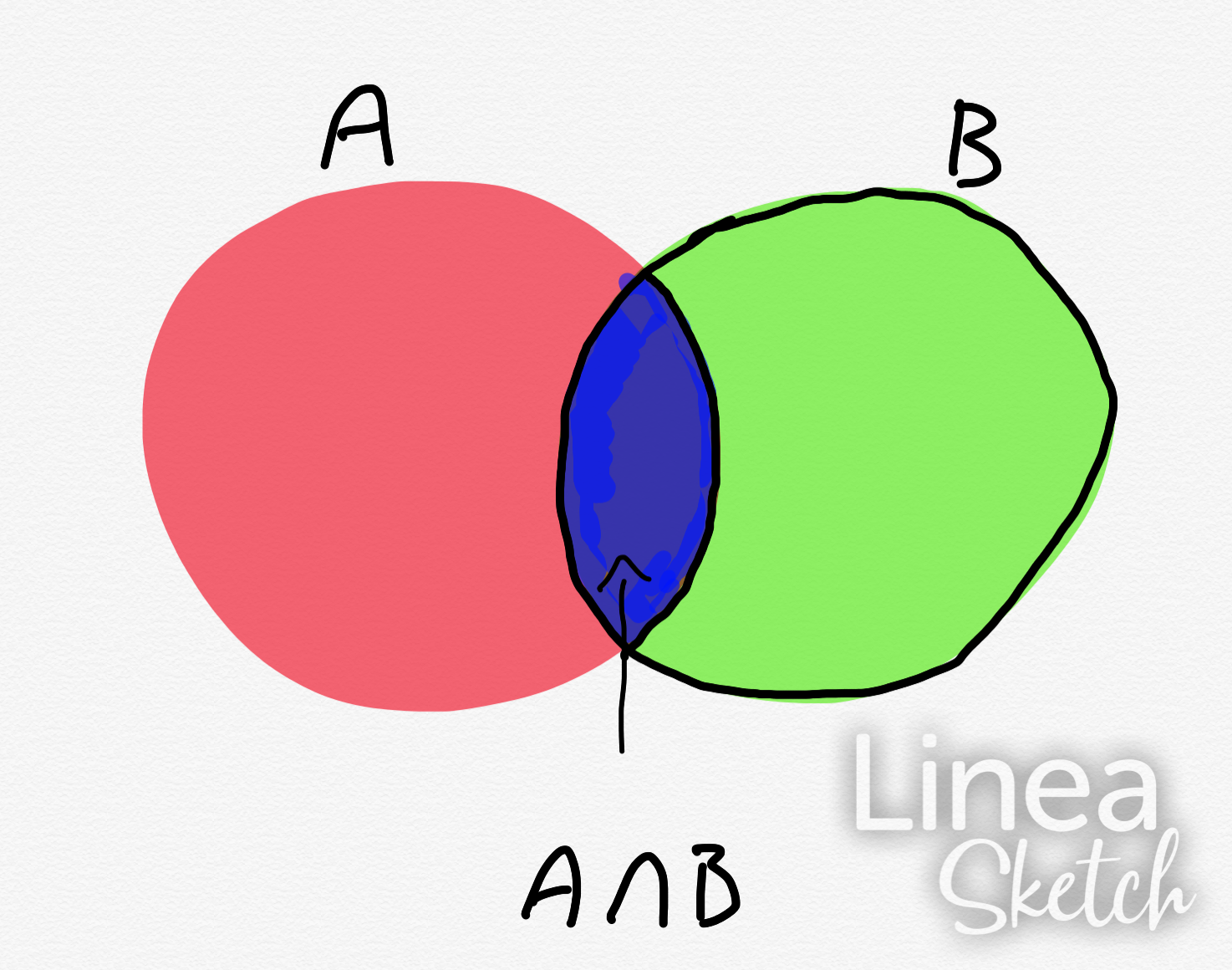
We know from the last class that Bayes formula is rooted in the geometry of the sample space. So we can use the fact that the intersection of two sets is associative, ie $ A\cap B = B\cap A $

From this we can derive the formula that is used throughtout the foundations of Bayesian Data Analysis
First we know
$$ P(A|B) = \frac{P(A\cap B)}{P(B)} $$and $$ \frac{P(B\cap A)}{P(A)}=P(B|A) $$
Which gives us
$$P(A\cap B) = P(A|B)P(B) $$and
$$P(B\cap A) = P(B|A)P(A) $$But, from our associative law
$$ P(A\cap B) = P(B\cap A) $$Hence that implies
$$ P(A|B)P(B) = P(B|A)P(A)$$ $$\implies $$$$ P(A|B) = \frac{P(B|A)P(A)}{P(B)} $$Or more conventially expressed,
$$ P(\theta | D) = \frac{P(D|\theta)P(\theta)}{P(D)} $$Example for a single data point
Example: A single data interpretation of this would be a Covid test. You just went to get a covid test today and it is positive. Whats the probability that you have Covid
Here, $\theta$ would be the belief you have covid and $D$ would be the data of recieving a positive result.
So $ P(\theta | D)$ is the probabilty of you having Covid given that you have a positive test.
That is equal to $P(D|\theta) P(\theta)$ divided by $P(D)$
Today, Feb 24th 2021, in the KC metro area the percentage of positive tests is 6.1%.
Looking up some efficacy on Covid Rapid tests, we can see that True positives are about 98.5% and False positives are about 2%
Theoretical meanings for distributional data spaces
Here, $\theta$ could be thought as the probability of a belief/hypothesis, and $D$ as an observed data set
This could be written as the probability of your belief given observed data is equal to the probability of that data given your belief times the probability of your belief divided by the total probability of overserving the data.
Moreover this can be expressed as
$$ \text{posterior} = \frac{\text{likelihood} \times \text{prior}}{\text{ marginal likelihood}} $$The prior , or $P(\theta)$, distributon is what the probability of our beliefs/hypothesis, before we start seeing the data
The likelihood, or $P(D| \theta)$, is the probability of the data given the belief/hypothesis that we have.
The posterior, $P( \theta|D)$, distribution of our beliefs/hypothesis after we see the data
And the marginal likelihood, $P(D)$ or normalized likelihood is the probability of the data under any circumstance
Lets look at an fair coin flipping
import matplotlib.pyplot as plt
import numpy as np
import seaborn as sns
from scipy import stats


%matplotlib inline
%config InlineBackend.figure_format='retina'
flips = 10
heads_prob = 0.5

Heads_flip = stats.binom(flips,heads_prob).rvs()
Tails_flip = flips-Heads_flip
print(Heads_flip,Tails_flip)
num_space = 100
prob_space = np.linspace(1/num_space,num_space/(num_space+1),num_space)

uniform_space = np.ones(num_space)*1/num_space
plt.plot(prob_space,uniform_space)
triangle_prob = np.minimum(prob_space,1-prob_space)
triangle_space = triangle_prob/triangle_prob.sum()
plt.plot(triangle_space)
plt.plot(prob_space,uniform_space)
plt.plot(prob_space,triangle_space)
We have the Priors
Now to find the likelihood given Heads and Tails
prob_space
def nCk(n,k):
    return np.math.factorial(n)/(np.math.factorial(n-k)*np.math.factorial(k))
prob_like = nCk(flips,Heads_flip)*prob_space**(Heads_flip)*(1-prob_space)**(Tails_flip)
prob_like
plt.plot(prob_space,prob_like,'.')
We have to find $P(D)$
prob_norm = np.sum(prob_space*prob_like)
Now all we have to do is apply Bayes Rule $$ P(\theta | D) = \frac{P(D|\theta)P(\theta)}{P(D)} $$
prob_prior = uniform_space

prob_post = prob_like*prob_prior
plt.plot(prob_space, prob_post)
plt.figure(figsize=(13,6))
plt.stem(prob_space,prob_prior, markerfmt=',')
plt.show()
plt.figure(figsize=(13,6))
plt.stem(prob_space,prob_like, markerfmt=',')
plt.show()
plt.figure(figsize=(13,6))
plt.stem(prob_space,prob_post, markerfmt=',')
plt.show()
plt.figure(figsize=(13,6))
plt.stem(prob_space,prob_prior, markerfmt=',')
plt.title('prior')
plt.show()

plt.figure(figsize=(13,6))
plt.stem(prob_space,prob_like, markerfmt=',')
plt.title('likelihood')
plt.show()

plt.figure(figsize=(13,6))
plt.stem(prob_space,prob_post, markerfmt=',')
plt.title('posterior')
plt.show()
lets put this into one cell and see the dynamics of this change
flips = 6
heads_prob = 0.5

Heads_flip = stats.binom(flips,heads_prob).rvs()
Tails_flip = flips-Heads_flip
print(Heads_flip,Tails_flip)


num_space = 100
prob_space = np.linspace(1/num_space,num_space/(num_space+1),num_space)
uniform_space = np.ones(num_space)*1/num_space

triangle_prob = np.minimum(prob_space,1-prob_space)
triangle_space = triangle_prob/triangle_prob.sum()

prob_like = nCk(flips,Heads_flip)*prob_space**(Heads_flip)*(1-prob_space)**(Tails_flip)

prob_prior = triangle_space

prob_norm = np.sum(prob_space*prob_like)

prob_post = prob_like*prob_prior/prob_norm


plt.figure(figsize=(13,6))
plt.stem(prob_space,prob_prior, markerfmt=',')
plt.title('prior')
plt.show()

plt.figure(figsize=(13,6))
plt.stem(prob_space,prob_like, markerfmt=',')
plt.title('likelihood')
plt.show()

plt.figure(figsize=(13,6))
plt.stem(prob_space,prob_post, markerfmt=',')
plt.title('posterior')
plt.show()